8 Scenario VII: binomial distribution, Gaussian prior
8.1 Details
In this scenario, we revisit the case from ScenarioVI, but are not assuming a point prior anymore. We assume \(p_C=0.3\) for the event rate in the control group. The parameter which can be varied is the event rate in the experimental group \(p_E\) and we assume that the rate difference \(p_E-p_C \sim \textbf{1}_{(-0.29,0.69)} \mathcal{N}(0.2,0.2)\).The restriction to the interval \((-0.29,0.69)\) is necessary to ensure that the parameter \(p_E\) does not become smaller than \(0\) or larger than \(1\).
In order to fulfill regulatory considerations, the type one error rate is still protected under the point prior \(\delta=0\) at the level of significance \(\alpha=0.025\).
Since effect sizes less than a minimal clinically relevant effect do not show evidence against the null hypothesis, we assume a clinically relevant effect size \(\delta =0.0\) and condition the prior on values \(\delta > 0\) in order to compute the expected power. We assume a minimal expected power of at least \(0.8\).
# data distribution and priors
datadist   <- Binomial(rate_control = 0.3, two_armed = TRUE)
H_0        <- PointMassPrior(.0, 1)
prior      <- ContinuousPrior(function(x) 1 /
                                  (pnorm(0.69, 0.2, 0.2) - pnorm(-0.29, 0.2, 0.2)) * dnorm(x, 0.2, 0.2),
                              support = c(-0.29, 0.69),
                              tighten_support = TRUE)

# define constraints on type one error rate and expected power
alpha      <- 0.025
min_epower <- 0.8
toer_cnstr <- Power(datadist, H_0) <= alpha
epow_cnstr <- Power(datadist, condition(prior, c(0.0, 0.69))) >= min_epower
8.2 Variant VII-1: Minimizing Expected Sample Size under Continuous Prior
8.2.1 Objective
Expected sample size under the full prior is minimized, i.e., \(\boldsymbol{E}\big[n(\mathscr{D})\big]\).
ess <- ExpectedSampleSize(datadist, prior)8.2.3 Initial Designs
For this example, the optimal one-stage, group-sequential, and generic two-stage designs are computed. The initial design for the one-stage case is determined heuristically and both the group sequential and the generic two-stage designs are optimized starting from the corresponding group-sequential design as computed by the rpact package.
order <- 7L
# data frame of initial designs
tbl_designs <- tibble(
    type    = c("one-stage", "group-sequential", "two-stage"),
    initial = list(
        OneStageDesign(200, 2.0),
        rpact_design(datadist, 0.2, 0.025, 0.8, TRUE, order),
        TwoStageDesign(get_initial_design(0.2, 0.025, 0.2, "two-stage", dist = datadist) )))
The order of integration is set to 7.
8.2.4 Optimization
tbl_designs <- tbl_designs %>%
    mutate(
       optimal = purrr::map(initial, ~minimize(
          ess,
          subject_to(
              toer_cnstr,
              epow_cnstr
          ),

          initial_design = .,
          opts           = opts)) )
8.2.5 Test Cases
To avoid improper solutions, it is first verified that the maximum number of iterations was not exceeded in any of the three cases.
tbl_designs %>%
  transmute(
      type,
      iterations = purrr::map_int(tbl_designs$optimal,
                                  ~.$nloptr_return$iterations) ) %>%
  {print(.); .} %>%
  {testthat::expect_true(all(.$iterations < opts$maxeval))}
## # A tibble: 3 × 2
## type iterations
## <chr> <int>
## 1 one-stage 21
## 2 group-sequential 642
## 3 two-stage 22550Furthermore, the type one error rate constraint needs to be tested.
tbl_designs %>%
  transmute(
      type,
      toer = purrr::map(tbl_designs$optimal,
                        ~sim_pr_reject(.[[1]], .0, datadist)$prob) ) %>%
  unnest(., cols = c(toer)) %>%
  {print(.); .} %>% {
  testthat::expect_true(all(.$toer <= alpha * (1 + tol))) }
## # A tibble: 3 × 2
## type toer
## <chr> <dbl>
## 1 one-stage 0.0251
## 2 group-sequential 0.0250
## 3 two-stage 0.0249The optimal two-stage design is more flexible than the other two designs, so the expected sample sizes under the prior should be ordered upwards as follows: optimal two-stage design < group sequential < one-stage. We additionally compare the simulated and theoretical outcomes of the sample size under the null.
essh0 <- ExpectedSampleSize(datadist, H_0)

tbl_designs %>%
    mutate(
        ess       = map_dbl(optimal,
                            ~evaluate(ess, .$design) ),
        essh0     = map_dbl(optimal,
                            ~evaluate(essh0, .$design) ),
        essh0_sim = map_dbl(optimal,
                            ~sim_n(.$design, .0, datadist)$n ) ) %>%
    {print(.); .} %>% {
    # sim/evaluate same under null?
    testthat::expect_equal(.$essh0, .$essh0_sim,
                           tolerance = tol_n,
                           scale = 1)
    # monotonicity with respect to degrees of freedom
    testthat::expect_true(all(diff(.$ess) < 0)) }
## # A tibble: 3 × 6
## type initial optimal ess essh0 essh0_sim
## <chr> <list> <list> <dbl> <dbl> <dbl>
## 1 one-stage <OnStgDsg> <adptrOpR [3]> 238 238 238
## 2 group-sequential <GrpSqntD> <adptrOpR [3]> 103. 161. 161.
## 3 two-stage <TwStgDsg> <adptrOpR [3]> 99.2 169. 169.8.3 Variant VII-2: Conditional Power Constraint
8.3.1 Objective
As in VariantVII-1, the expected sample size under the full prior is minimized.
8.3.2 Constraints
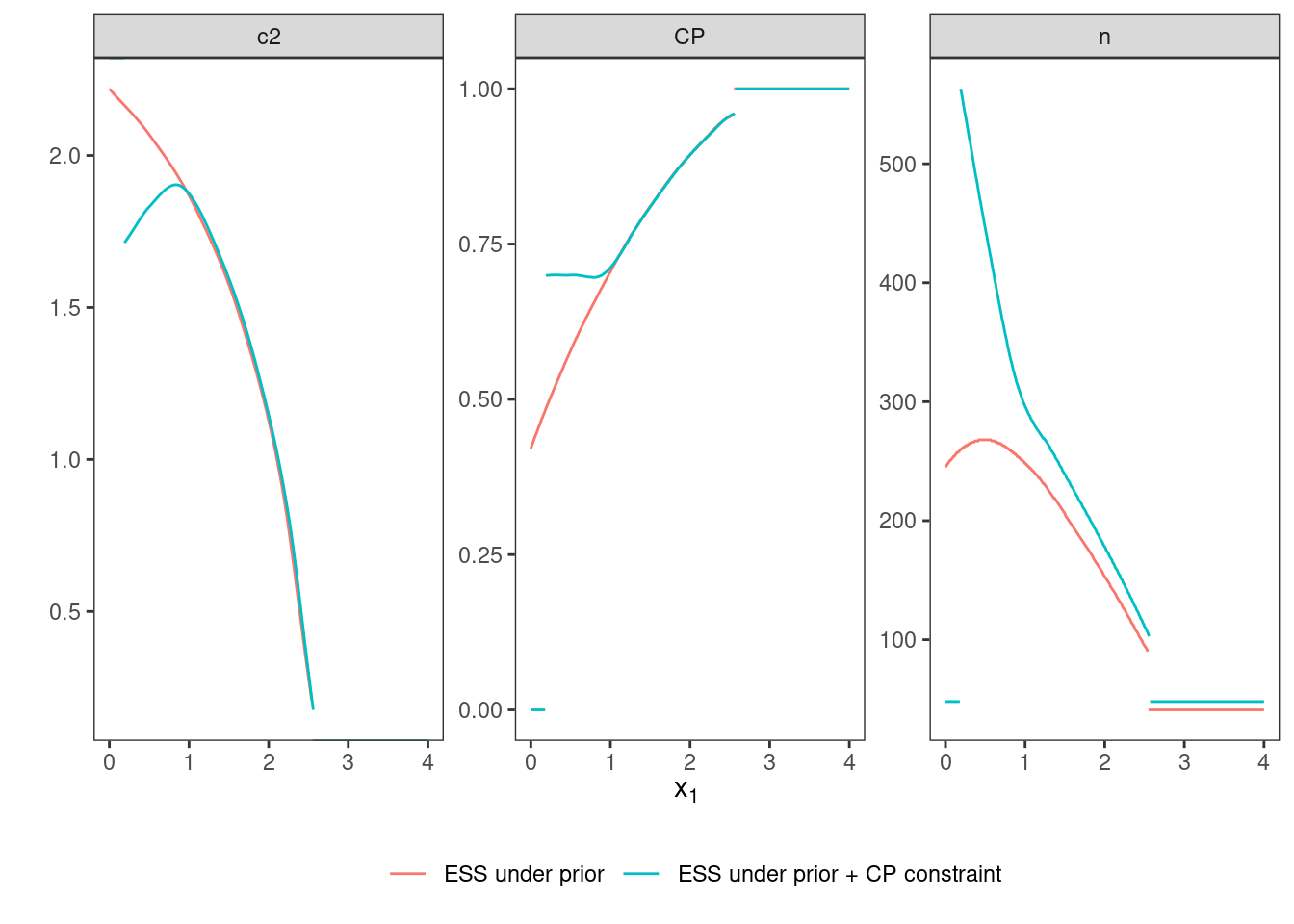
In addition to the constraints on type one error rate and expected power, a constraint on conditional power to be larger than \(0.7\) is included.
cp       <- ConditionalPower(datadist, condition(prior, c(0, 0.69)))
cp_cnstr <- cp >= 0.78.3.4 Optimization
opt_cp <- minimize(
        ess,
        subject_to(
            toer_cnstr,
            epow_cnstr,
            cp_cnstr
        ),
        initial_design = tbl_designs$initial[[3]],
        opts = opts
)
8.3.5 Test Cases
As always, we start checking whether the maximum number of iterations was reached or not.
testthat::expect_true(opt_cp$nloptr_return$iterations < opts$maxeval)
print(opt_cp$nloptr_return$iterations)
## [1] 17551The type one error rate is tested via simulation and compared to the value obtained by evaluate().
tbl_toer <- tibble(
  toer     = evaluate(Power(datadist, H_0), opt_cp$design),
  toer_sim = sim_pr_reject(opt_cp$design, .0, datadist)$prob
)

print(tbl_toer)
## # A tibble: 1 × 2
## toer toer_sim
## <dbl> <dbl>
## 1 0.0250 0.0249testthat::expect_true(tbl_toer$toer <= alpha * (1 + tol))
testthat::expect_true(tbl_toer$toer_sim <= alpha * (1 + tol))The conditional power is evaluated via numerical integration on several points inside the continuation region and it is tested whether the constraint is fulfilled on all these points.
tibble(
    x1 = seq(opt_cp$design@c1f, opt_cp$design@c1e, length.out = 25),
    cp = map_dbl(x1, ~evaluate(cp, opt_cp$design, .)) ) %>%
  {print(.); .} %>% {
      testthat::expect_true(all(.$cp >= 0.7 * (1 - tol))) }
## # A tibble: 25 × 2
## x1 cp
## <dbl> <dbl>
## 1 0.190 0.699
## 2 0.288 0.700
## 3 0.387 0.700
## 4 0.486 0.700
## 5 0.585 0.700
## 6 0.684 0.698
## 7 0.783 0.697
## 8 0.882 0.699
## 9 0.981 0.709
## 10 1.08 0.725
## # ℹ 15 more rowsDue to the additional constraint, this variant should show a larger expected sample size.
testthat::expect_gte(
    evaluate(ess, opt_cp$design),
    evaluate(
        ess,
        tbl_designs %>%
            filter(type == "two-stage") %>%
            pull(optimal) %>%
            .[[1]] %>%
            .$design )
)